Tutorial

Introduction

In this chapter we will see a simple and practical use of rNAV with a small dataset.

You can find the data used in this tutorial in the directory .../rNAV2.0/samples/

Import data

Launch rNAV

The default installation mode install a shell script in the directory .../rNAV2.0/rNAV If you chose a specific install path, you could alwyas find a rNAV executable file in your_install_dir/install/bin/rNAV You should see the main window :

Load or import data

CLick on the green plus button to open the Load or import window and activate the third tab called Import from genome file:

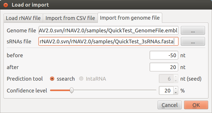
Choose the QuickTest_GenomeFile.embl located in the samples directory as genome file:

rNAV2.0/samples/QuickTest_GenomeFile.embl

Choose the MycoplasmaCapricolum_6sRNAs.fasta located in the samples directory as sRNAs file:

rNAV2.0/samples/QuickTest_3sRNAs.fasta

Keep before and after values set on -50 and 20. Leave Prediction tool set to ssearch and set Confidence level whatever you want. Click on OK. You should obtain a first network looking like this:

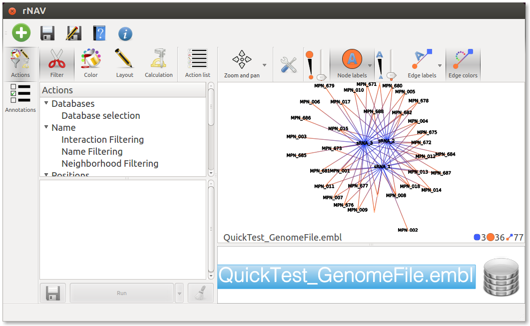
Perform actions on the network

Position clustering

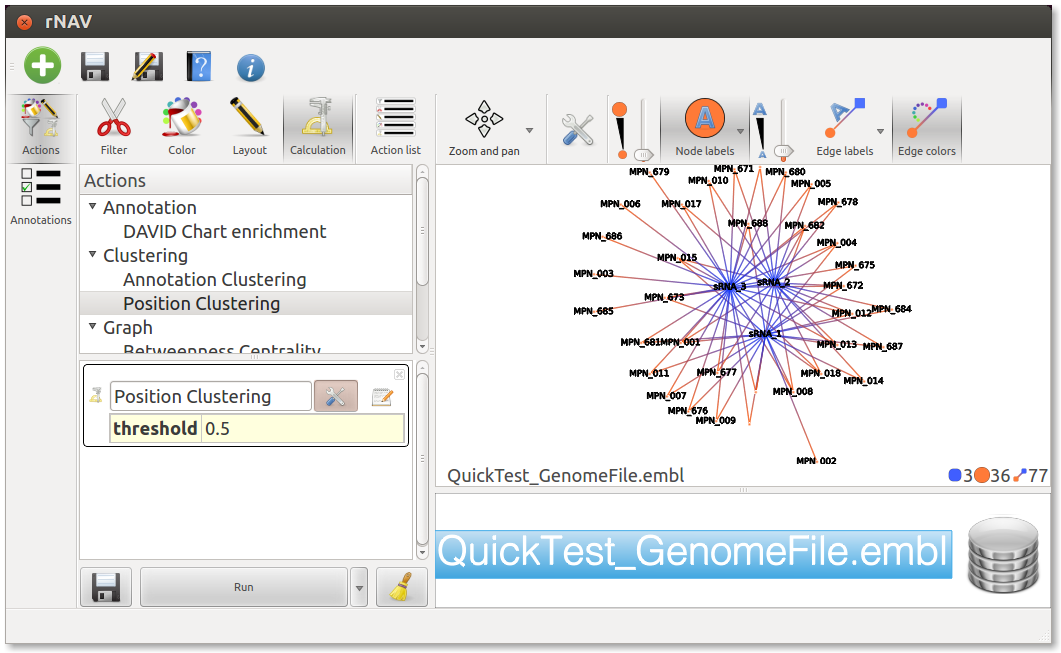
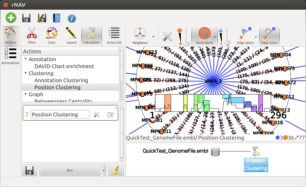
At the top of the Action management widget, click on the Calculation icon, and in the underlaying list, double click on Position clustering. This will create an entry called Postion Clustering in the list below. At this point you can set the threshold by clicking the tools button next to Position Clustering or leave it to the default value. Finally, click on the Run button at the bottom of this list to perform the action.

Neighbors interactor

Use it to explore the network. Click on the Interaction tools selector (which displays the default interactor Zoom and pan ) and choose Neighbors

Now you can explore each sRNA by clicking on the blue node representing it. Use the mouse wheel to zoom. If nodes do appear too small, use Nodes size tool |nodes_size| to enlarge them.

DAVID[1] chart enrichement

Enrich your network with functional biological data from many public databases through DAVID webservice.

First select the root graph, named QuickTest_GenomeFile.embl in the Action history widget so that the enrichement will be applied to the whole network.

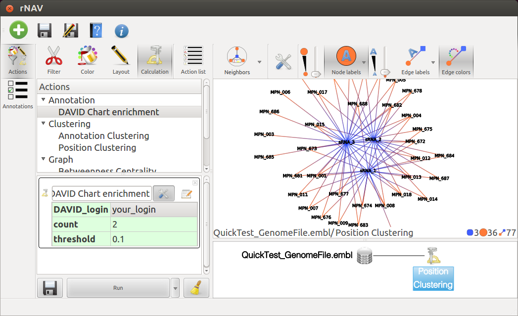
To start fetching datas from DAVID webservice, just double click on the DAVID Chart enrichement action from the action list and open parameters setting by clicking on the Tools button.

Fill in your DAVID login if you don’t have one, go and register at

http://david.abcc.ncifcrf.gov/webservice/register.htm Then click on Run, fetching time depends on number of sRNAs.

Activate Annotations list to see the results. You can also display the annotations on the edge labels (Choose Short annotations for better visualization).

Annotation Clustering

This action will cluster edges with close annotations.

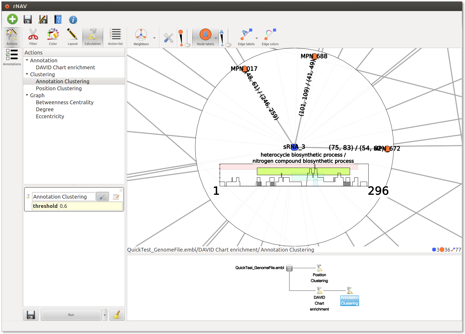
The result should be observed with the Neighbors interactor. Each colored box represents a cluster of annotations, meaning a group of edges with close annotations. You can read the whole annotations list of the cluster by hovering this box. You will also see which edges are involved in the cluster. The little gray box under the frequency curve show (such as the frequency curve) the position of the predicted interaction on the sRNA (or mRNA if the center node of the interactor is a mRNA).

Multiple View

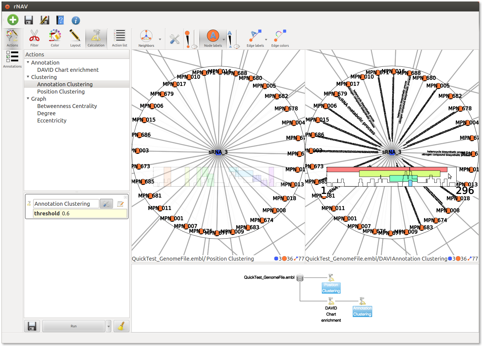
rNAV can split his visualization widget to display multiple graph.

To do so, select multiple states in the Action history widget by clicking on them while holding down the Ctrl key.

All views are synchronized together. Moreover, you can now apply the same action (or even action list) on all the subgraphs displayed

In the screenshot below, you can see both Position clustering and Annotation clustering displayed together.

Finally

You can try other actions or a bigger network with a whole genome using the two others files provided in the samples directory:

• .../rNAV2.0/samples/MycoplasmaCapricolum.embl
• .../rNAV2.0/samples/MycoplasmaCapricolum_6sRNAs.fasta

[1] D. W. Huang, B. T. Sherman, and R. A. Lempicki. Systematic and integrative analysis of large gene lists using david bioinformatics resources. Nat Protoc, 4(1):44–57, 2009.